The Distribution of distributions

Why is the Distribution of distributions important?

Likeliness theory assumes that distributions are spread out evenly over the underlying set; that they're not concentrated in the top-right-hand corner, for example.

We can devise our algorithms so that the distributions we generate are spread out evenly. The question, though, is whether real-life distributions are like that. Maybe real-life distributions really are concentrated in the top-right-hand corner.

It is important to likelinesses, and to other branches of mathematics, that we check on this if we can.

The process

It is easy to visualise the process we would have to go through to investigate this:-

- choose a population (degree and underlying set)

- search for real-life examples

- compare the distribution of those real-life examples with what we would expect it to be if they were evenly spread out.

Choosing a degree and underlying set

The degree and underlying set need to be a common enough combination to produce sufficient examples for the collection of data within a reasonable time.

For example, it would not be wise to try collecting real-life examples of unimodal distributions of degree 33 and mode 12; I don't think I have ever seen one of those, so collecting a sufficiently large sample could take several lifetimes.

Authors have a prediliction for publishing their data in rank order. This introduces bias which renders almost every underlying set unusable.

This prediliction for publishing in rank order ceases to be a problem if we are actually collecting ranked data. So we shall collect examples of R(N) data for some N.

There is plenty of "top 10" data available, so our first thoughts would be to use that.

"top 10" data is not the same as R(10) data.

Tables of top 10 data do not just take data of degree 10 and publish it. They take data of degree at least 10, ignore everything from rank-position 11 onwards and then publish what's left. This process, which Ranked Distributions on Finite Domains (RDoFD) calls S(N) reduction, introduces an unwanted distortion. There is a solution, which the same publication calls R(N) reduction

.

The use of R(N) reduction

The definition of R(N) reduction is quite abstract but it has a simple practical interpretation. For each distribution, r, subtract r(N+1) from each of r(1),...,r(N). Normalisation, by dividing the resulting terms throughout by their sum, then gives the R(N) reduction of r.

For example, if r is the degree 5 distribution

(0.34, 0.24, 0.20, 0.14, 0.08)

then its R(3) reduction is found by firstly calculating

(0.34-0.14, 0.24-0.14, 0.20-0.14)=(0.20,0.10,0.06)

and then normalising by dividing throughout by 0.20+0.10+0.06=0.36 to produce (to 2 dp)

(0.56, 0.28, 0.17)

For top 10 data, we can find the R(9) reductions by subtracting r(10) from each of r(1),...r(9) and then dividing throughout by their sum. This will give a set of distributions of degree 9 which may be treated as if they were our original sample: if there is any bias then it would have been inherited from the un-reduced data rather than introduced by the reduction process.

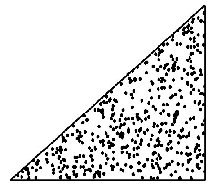
Whilst we are at it, we may as well find the R(3) reductions, since it is possible actually to see how degree 3 distributions are distributed over R(3) or S(3), as appropriate: R(3) and S(3) are both normal, everyday triangles.

The data

We will be investigating whether the distribution of all real-life distributions follows our expectations. So we must not allow personal bias to affect our choice of distributions: any top 10 distribution must be accepted.

500 top-10 distributions were collected. The following gives a flavour of them.

The results

R(9) reductions

Because there were 500 distributions in the sample, there are 500 R(9) Reductions and therefore, for each i=1,...,9, there are 500 values of r(i), each r being an R(9) Reduction.

For each i:-.

1.Twenty cells were chosen in [0,1] such that the smallest of those 500 values was in the first cell, and the largest was in the 20th. The proportion in each cell was then found: these are shown in the following animation as the dots.

2. For each cell, 'Great Likelinesses' was used to find the likeliness, over R(9) and given 0, that r(i) would be in that cell. These likelinesses are shown as the curve, and represent the theoretical proportions.

• The curve gives the theoretical values if the data were distributed evenly over R(9)
• The dots show the actual data from the sample.