Lovegrove Mathematicals
"Probabilities are likelinesses over singleton sets"
Likeliness terminology
The Degree
- A coin is of degree 2;
- A die is of degree 6;
- A pack of cards is of degree 52;
- The days of the week are of degree 7.
The degree is the number of possibilities that something (tossing a coin; rolling a die; drawing a card) may take. To enable a coherent theory to be developed, the possibilities/classes are labelled 1,2,...,N where N is the degree.
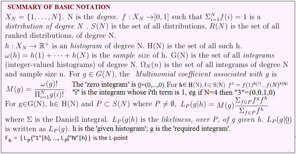
The set {1,...,N} is denoted by XN. This is the domain of definition for distributions and histograms of degree N.
Distributions
A distribution of degree N is a function f:XN→]0,1] such that f(1)+…+f(N)=1
It is usual to represent the distribution f by the ordered N-tuple ( f(1), ... ,f(N) ).
The set of all distributions of degree N is denoted by S(N).The symbol SN is more usual, but to use that here would result in an inelegant subscripted subscript -which is difficult to typeset in a clear and legible way.
If f∈S(N) then f is injective if [i≠j] ⇒ [f(i)≠f(j)]. The set of non-injective elements of S(N) has measure zero and so may be safely ignored: the description of various algorithms as producing injective distributions is for the sake of technical precision only, and has no practical or theoretical consequences.
Histograms
An histogram of degree N is any function h:XN→[0,∞[
The set of all histograms of degree N is denoted by H(N).
The sample size of h is ω(h)= h(1)+...+h(N).
When writing out the histogram h we normally just write out the values of the h(i) as an ordered N-tuple. For example, (1.25, 2.13, 4.87, 8.92)
Integrams
An integram of degree N is an histogram of degree N which has only integer values. (1, 2) is an integram; (1, 2.0) is not. The most important integram is the zero integram 0 for which all values are zero.
The set of all integrams of degree N is denoted by G(N). The set of all integrams of degree N and sample size n is ΩN(n), so if g∈G(N) then g∈ΩN(ω(g)).
We denote the integram g(i)=1, g(j)=0 for j≠i by ''i''N (the quote marks are part of the notation). Because the degree is normally obvious from the context, this will usually be written as ''i''For those familiar with vector notation, this is the same as the bolded i used to denote an unit vector in the direction of the i-axis. That notation is impossible to write by hand and so must be the worst piece of notation ever devised.
For example, if the degree is 6 then "2"="2"6=(0,1,0,0,0,0)
If g∈G(N) the Multinomial coefficient associated with g is given by
(Because the denominator contains the term g(i)! then g(i) must be an integer. Since this is the case for all i, g does have to be an integram, not just an histogram.)
Relative Frequencies
Let h∈H(N) with ω(h)>0. Then we define RF(h) to be the relative frequencies of h, that is RF(h)(i)= h(i)/ω(h). An alternative notation for RF(h)(i) is RF(i|h), the relative frequency of i given h.
If h1, ..., hK∈H(N) then, for i∈XN:-
- Provided at least one ω(hj)>0,so that ω(h1)+...+ω(hK)≠0 we
define the Mean Relative Frequency of i to be
 .
.
An alternative name for this is the Global Relative Frequency of i.
- Provided no ω(hj)=0, we define the Mean of the Relative Frequencies of i to be
Convex and concave sets
A set, P, is convex if, no matter which two points we select in P, the straight line segment joining them is wholly in P. A set which is not convex is called concave, but many authors prefer the term non-convex.
The core (some prefer the term convex hull) of a set is its smallest convex superset. It follows from the definition that a convex set is its own core.
Core(P) is important because the mean of any number (not necessarily finite) of elements of P always lies in Core(P). In particular, if P is convex then the mean lies in P, but if P is concave then that mean might not be in P.
Symmetry
If P⊂S(N) then P will be said to be (i,j)-symmetric if P contains f(i,j) whenever P contains f, where f(i,j) is that distribution which is obtained from f by interchanging f(i) and f(j).
The histogram h is (i,j)-symmetric if h(i)=h(j).
P is symmetric if it is (i,j)-symmetric for all i,j∈XN.
h is symmetric if it is (i,j)-symmetric for all i,j∈XN. That is, if it is a constant histogram.
Likeliness of an Integram
Let P be a non-empty subset of S(N), g∈G(N) and h∈H(N) then we define the Likeliness, over P, of g given h by
h is called the given histogram (often an integram, but it doesn't have to be), and g is the required integram. P is the underlying set. (g+h) is the objective histogram. It is often the case that it is the objective histogram that is specified, and the required integram is then found by subtracting the given histogram
∫ is the Daniell integral, which can be thought of as summation on a finite set but as the Riemann integral when that is required.
Provided no confusion results, we
- write LP(i|h) rather than LP("i"|h);
- write LP(g) rather than LP(g|0).
The L-point is the point (distribution) in S(N) with co-ordinates
( LP(1|h), ..., LP(N|h) ). Associated with this is the function
which will be often used on this site to plot graphs. When doing this, we shall sometimes use the alternative notation Average(P) rather than LP.
Likeliness of a set of distributions
If Pis an underlying set in (ie. a non-empty subset of) S(N), V⊂S(N) and h∈H(N) then we define the Likeliness, over P, of V given h by
When h=0, we write LP(V) rather than LP(V|0)
A fundamental difference between the likeliness of an integram and the likeliness of a set of distributions is that the former cannot be 0 but the latter can (if V and P do not intersect). Similarly, the likeliness of an integram cannot be 1 (except in the degenerate case N=1), but that of a set of distributions can (if P⊂V).
If P is a singleton set, P={f}, then LP(V|h) can be only 0 (if f∉V) or 1 (if f∈V) and is equivalent to the characteristic function of V.