Lovegrove Mathematicals
"Dedicated to making Likelinesses the entity of prime interest"
Lovegrove Mathematicals
"Dedicated to making Likelinesses the entity of prime interest"
There are (at least) two interpretations of multimodality. These require exactly the same information; it's just the way that the algorithms treat that information which varies. One is a general definition, the other is meaningful only under narrower (but arguably more realistic) conditions.
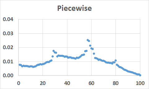
In the general approach, multimodal distributions are built up as linear combinations of 'mini' unimodal distributions, and the underlying set is the set of all such linear combinations. The concept, of a multimodal distribution being constructed from unimodal pieces, is usually called piecewise multimodality, or (confusingly) piecewise unimodality.
In the narrower interpretation, no multimodal distributions are produced. All the distributions are unimodal but selected from different populations. It is the combination of those different populations which gives the multimodal effect. There is no general name for this approach, so it will here be called systemical unimodality.
Each multimodal distribution is defined in terms of a number of 'pieces', each of which consists of
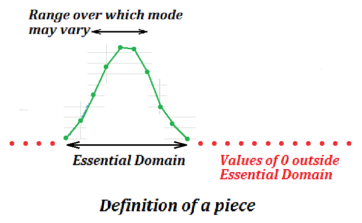
The essential domains may overlap. They do not have to overlap, but their union must cover XN.
The final distribution is formed by taking a linear combination of those (extended) unimodal distributions.
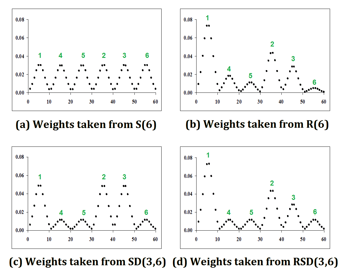
The weights used when forming the linear combination are not usually specified as such. What is specified is a set of distributions from which they are to be chosen. If there are p pieces then this set will be a subset of S(p); Great Likelinesses, for example, allows the use of one of the sets S(p), R(p), SD(c,p) for some c, RSD(c,p). The computer takes a different choice of weights from the specified set each time that it constructs a multimodal distribution. Also needing to be specified is the order in which these weights are to be applied to the pieces -for example, they do not have to be applied left-to-right.
The following figures show the effect of changing the set of weights. The order in which the weights are applied is indicated by the green numerals.
The pieces and weights are specified exactly as for the piecewise approach. However, if each essential domain is XN then systemical multimodality becomes well-defined and so can be used.
In this, a random selection of a piece is made, and an unimodal distribution is selected on that piece. That distribution is then used as an element of the underlying set.
No linear combinations are produced, so the weights are not used as coefficients as in the piecewise approach. Instead, they are used as probabilities-of-selection for the pieces, when determining which piece to use as in the previous paragraph..
Each distribution produced by the algorithm is unimodal (and, because its essential domain is XN, is of degree N). The multimodality comes from the combination of those unimodal distributions.
As the essential domains all go from 1 to 100, we have the choice of which concept of multimodality to use. In the following, we shall be carrying out two analyses, firstly using one concept then the other, so that we can compare the two.
The individual distributions are unimodal. The multimodal effect comes from their being taken from 4 different populations. The Figure shows one distribution on each of the pieces; each distribution is a member of the underlying set.
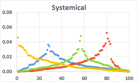
Each individual distribution is multimodal.
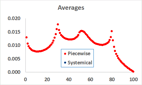
The two graphs of average values (here, the averages are of 750,000 distributions each) are identical. This is bound to be the case, and the explanation is not deep. If we ignore the difference in terminology but look at the detailed arithmetic then it turns out that we do exactly the same calculations in both cases. The terminology used to describe those calculations differs, but the arithmetic is identical. Since the arithmetic is identical, we obtain the same end-result in both cases.
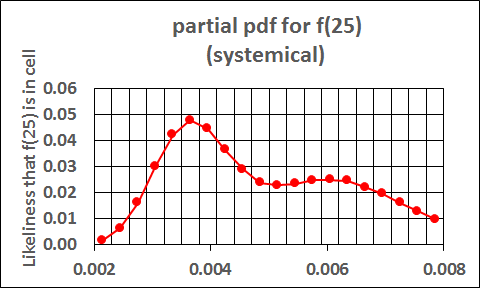
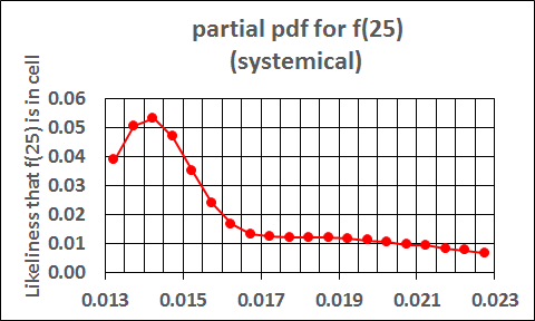
Using f(25) as an example, the following animation compares the pdfs for the systemical and piecewise definitions.
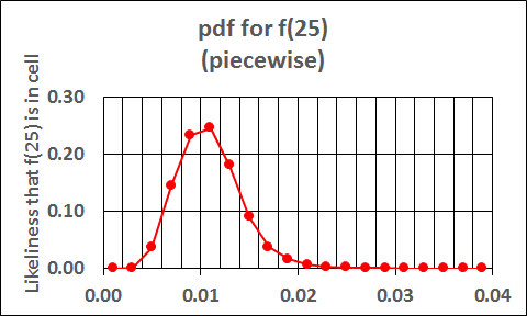
There is, though, a problem: we would expect the pdf for the systemical case to have four modes (one for each population), not just two. The difficulty, here, is due to the resolution: the diagram is too coarse to show all four modes.
If we improve the resolution by zooming in, as in the next two figures, then we can see that there are four modes (there is a local mode at just under 0.019)