Lovegrove Mathematicals
"Dedicated to making Likelinesses the entity of prime interest"
Lovegrove Mathematicals
"Dedicated to making Likelinesses the entity of prime interest"
A distribution is unimodal if it has precisely one mode.
The basic idea is to start with r∈R(N)=the set of ranked distributions of degree N and then permute its values to produce an element of M(m,N). We do this by firstly placing r(1), then r(2) etc.
Clearly, r(1) must be placed at m.
Since the final distribution is to be unimodal, r(2) must then be placed at either (m-1) or (m+1), since any gap would eventually give rise to a dip which would spoil the unimodality. This generalises; at each step, all of the already-placed values must form a contiguous block with the next value being placed immediately adjacent to it at either end. We need to decide which end.
If the block extends all the way to either end of XN then there is no decision to be made: all of the remaining values go at the other end of the block.
Otherwise, let there be L unfilled places to the left
of the block and R to the right, with neither L nor R being 0. There are then
L+RCL ways to choose
the L values to fill the spaces to the left. In
L+R-1CL-1
of these, the value we are seeking to place will be to the left of the block -
a proportion of L+R-1CL-1
/ L+RCL
, which is
 : so we
toss the
coin
: so we
toss the
coin
 . If
the coin comes down "H" then we put the next value to the left; if it comes down
"T" then we put the next value to the right.
. If
the coin comes down "H" then we put the next value to the left; if it comes down
"T" then we put the next value to the right.
There are N-1Cm-1 unimodal permutations of r∈R(N) which have a mode at m. So we can count the total number which have a mode at A, ..., B, and thus the proportion of those which have a mode at any specific value. We then use RANDOM to select one of them in accordance with those proportions and then construct a unimodal distribution with that specific mode.
The general shape of an unimodal distribution as being a maxium at the mode and then dying away as we move away from the mode is a property of local modes, in particular strong local modes; it is not a property of global modes. If you have read about the meaning of 'mode' then you would have seen this.
There is a tendency for mathematical texts to give the impression that a typical unimodal distribution is bell-shaped (that is, it has tails and a rounded peak). This impression, which is far from correct regardless of whether we are using Local or Global modes, is due to the use of equations to represent distributions: there is no obvious equation for unimodal distributions which does not force a bell shape.
But being bell-shaped is such a harsh condition to satisfy that in reality it just about never occurs; certainly, there is nothing in the definition of "unimodal" which requires, or even suggests, a bell shape.
This is a random selection of elements of M(29). None of them is bell-shaped.
The next diagram shows the likelinesses of i=1,...,29 for distributions from the underlying set M(6,29). The graph shows what local unimodal distributions look like on average with a specific mode: the peak is very sharp, and is of a type which cannot be easily represented by a formula.
.png)
A bell shape can, however, occur on average if we do not specify a precise value for the mode.
As we begin to allow the mode to take on a range of values, so the mean distribution begins to take on a more rounded shape. Here, with the mode allowed to vary from 3 to 10, that is with the underlying set M(3 to 10,29),we can see the beginnings of a rounding to the left of the peak.
.png)
Use of the underlying set M(1 to 13,29) brings further rounding at the peak.
.png)
With the underlying set M(1 to 16,29), the mode is ranging over most of the domain and the graph is looking almost bell-shaped.
.png)
Finally, with the underlying set M(29) a full, symmmetric bell-shape has developed.
.png)
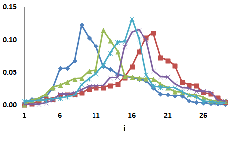
The following animation is another way to see the development of a bell-shape as vagueness about the mode increases. Notice how the bell-shape appears to have developed once the underlying set reaches about M(1 to 21, 29), with there being no noticeable change from there on.
Diagrams such as these show that a bell-shape can arise because of lack of precise information about the mode. The more widely we allow the mode to range in our analyses, the more bell-shaped the pdf becomes.
A bell-shape can also arise -at least, approximately enough for us not to be able to detect the difference- if we take samples from several unimodal distributions with different modes.
For such reasons, although Great Likelinesses will allow the underlying set to be a set of bell-shaped distributions, the manual recommends that that should not be done; it would be better to use a set of unimodal distributions with a vague mode.
Even though I would not now recommend the use of bell-shaped distributions to form the underlying set, they were what started my interest in this subject. I originally graduated in civil engineering, and began my professional career working in the concrete lab, where I literally swept the floor, oiled the moulds and made the cubes. I was occasionally allowed to sit-in on meetings, and it was there that I first encountered the problem of whether concrete strengths were Normally or Log-Normally distributed. Although I went off and did research/management in other areas, at the other end of my working life I found myself on an international research committee which was concerned with matters concrete. Again, the problem of concrete strengths arose although, by then, Weibull 2-point had been thrown in, as well. It struck me that although the engineering science suggested a bell-shape it didn't go any deeper than that: "bell-shaped" was the best that it could do. No wonder all the candidate distributions were bell-shaped but there was no agreement about which one was best: the fundamental science did not go into enough detail to discriminate between them. So I began to wonder if there was a method of analysis which was based on only the assumption of bell-shaped. Then I hit retirement.
It is vital that you read about the meaning of 'mode' before proceeding with this page.
This site uses strong local modes unless stated otherwise